PyTorch正则化和批标准化
Regularization-正则化:减小方差的策略
误差可分为解为:偏差,方差与噪声之和,即误差=偏差+方差+噪声之和;
偏差:度量了学习算法的期望预测与真实结果的偏离程度,即刻画了学习算法本身的拟合能力;
方差:度量了同样大小的训练集的变动所导致的学习性能的变化,即刻画了数据扰动所造成的影响;
噪声:表达了在当前任务上任何学习算法所能达到的期望泛化误差的下界。
简而言之,偏差是指在所有训练数据上训练得到的模型性能和在真实数据上表现的差异,方差是指模型在训练集和验证集(测试集)上的差异,方差重点在于不同数据集;噪声则是指给定的数据集(其可能存在噪声),那么当前数据集的数据质量已经决定了学习性能的上限,学习的目标就是尽可能的接近这个上限。
举个简单的例子,我们使用一个复杂的函数去拟合下面的数据点集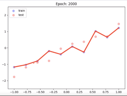
其能够完美的拟合所有训练集的点,但是测试集表现非常差,这就是高方差的典型例子,正则化就是为了降低方差。
L1和L2正则项
前面我们已经知道:目标函数=代价函数+正则项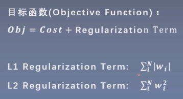
那么当我们想要优化目标函数时(使目标函数最小),同时也要优化正则项的值,L1和L2的正则化方式就是权重值计算方式不同,这里为了使得正则项的值尽可能小,所以要求权重矩阵的值也会尽可能的小,从而使得模型不会过于复杂。
L2正则项:weight decay(权值衰减)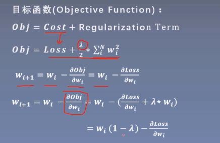
在pytorch中,加入L2正则项后的权重值的更新与不带正则项相比,会先对w乘以(1-λ),而0<λ<1,所以相当于对权重进行了一个缩小的操作,所以L2正则项被叫做权值衰减。
下面我们用代码展示一下使用weight_decay和不使用的区别1
2
3
4
5
6
7
8
9
10
11
12
13
14
15
16
17
18
19
20
21
22
23
24
25
26
27
28
29
30
31
32
33
34
35
36
37
38
39
40
41
42
43
44
45
46
47
48
49
50
51
52
53
54
55
56
57
58
59
60
61
62
63
64
65
66
67
68
69
70
71
72
73
74
75
76
77
78
79
80
81
82
83import matplotlib.pyplot as plt
import torch
import torch.nn as nn
n_hidden = 200
max_iter = 2000
disp_interval = 200
lr_init = 0.01
def gen_data(num_data=10, x_range=(-1, 1)):
w = 1.5
train_x = torch.linspace(*x_range, num_data).unsqueeze_(1)
train_y = w*train_x + torch.normal(0, 0.5, size=train_x.size())
test_x = torch.linspace(*x_range, num_data).unsqueeze_(1)
test_y = w*test_x + torch.normal(0, 0.3, size=test_x.size())
return train_x, train_y, test_x, test_y
train_x, train_y, test_x, test_y = gen_data(x_range=(-1, 1))
class MLP(nn.Module):
def __init__(self, neural_num):
super(MLP, self).__init__()
self.linears = nn.Sequential(
nn.Linear(1, neural_num),
nn.ReLU(inplace=True),
nn.Linear(neural_num, neural_num),
nn.ReLU(inplace=True),
nn.Linear(neural_num, neural_num),
nn.ReLU(inplace=True),
nn.Linear(neural_num, 1),
)
def forward(self, x):
return self.linears(x)
net_normal = MLP(neural_num=n_hidden)
net_weight_decay = MLP(neural_num=n_hidden)
optim_normal = torch.optim.SGD(net_normal.parameters(), lr=lr_init, momentum=0.9)
# 区别就在于weight_decay参数,λ=1e-2
optim_wdecay = torch.optim.SGD(net_weight_decay.parameters(), lr=lr_init, momentum=0.9, weight_decay=1e-2)
loss_func = torch.nn.MSELoss()
for epoch in range(max_iter):
# forward
pred_normal, pred_wdecay = net_normal(train_x), net_weight_decay(train_x)
loss_normal, loss_wdecay = loss_func(pred_normal, train_y), loss_func(pred_wdecay, train_y)
optim_normal.zero_grad()
optim_wdecay.zero_grad()
loss_normal.backward()
loss_wdecay.backward()
optim_normal.step()
optim_wdecay.step()
if (epoch + 1) % disp_interval == 0:
test_pred_normal, test_pred_wdecay = net_normal(test_x), net_weight_decay(test_x)
# 绘图
plt.scatter(train_x.data.numpy(), train_y.data.numpy(), c='blue', s=50, alpha=0.3, label='train')
plt.scatter(test_y.data.numpy(), test_y.data.numpy(), c='red', s=50, alpha=0.3, label='test')
plt.plot(test_x.data.numpy(), test_pred_normal.data.numpy(), 'r-', lw=3, label='no weight decay')
plt.plot(test_x.data.numpy(), test_pred_wdecay.data.numpy(), 'b--', lw=3, label='weight decay')
plt.text(-0.25, -0.15, 'no weight decay loss={:.6f}'.format(loss_normal.item()),
fontdict={'size': 15, 'color': 'red'})
plt.text(-0.25, -2, 'weight decay loss={:.6f}'.format(loss_wdecay.item()),
fontdict={'size': 15, 'color': 'red'})
plt.ylim(-2.5, 2.5)
plt.legend(loc='upper left')
plt.title("Epoch: {}".format(epoch+1))
plt.show()
plt.close()
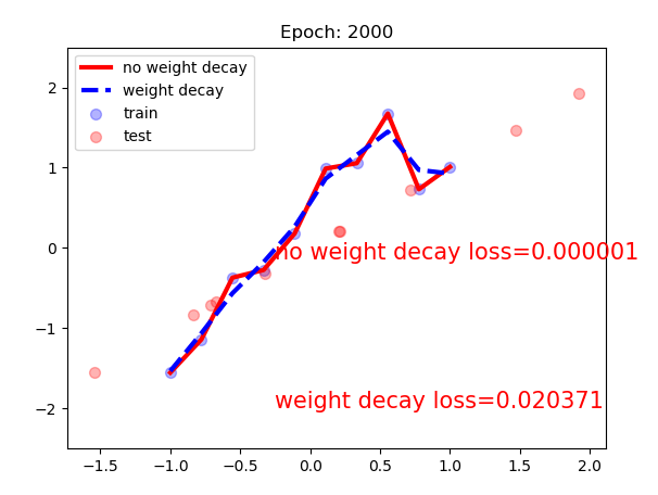
可以看到如果不使用weight decay,损失降到一个非常非常小的值,已经过拟合了,在测试集上效果并不好;而加了weight decay之后,损失相比之前略大一些,但是在这个例子中依然是过拟合的,不过相比之前略有缓解,蓝色的曲线相比红色也稍微平缓一些,也就是说仅靠weight decay并不是都能显著的优化所有问题。
Dropout:随机失活
功能:避免结果过度依赖某个神经元。通过设置参数p,确定网络中被舍弃的神经元数量,如p=0.3,有30%的神经元会失活(被舍弃)。
参考文献:《Dropout:A simple way to prevent neural networks from overfitting》
在以前的这一篇博客中也有对正则化进行解释:https://forchenxi.github.io/2021/01/26/dl-basics/
在这片博客中也有记录,由于训练时使用了dropout, 而测试时没有单元被舍弃,而该层的输出值需要按 dropout 比率缩小,因为这时比训练时有更多的单元被激活,需要加以平衡。
比如p=0.3,那么需要将输出值乘以(1-p)=0.7才可以与训练时一致,而pytorch实际实现时,在训练时权重均乘以[1/(1-p)],即除以(1-p)来增大权重,从而在测试时不需要再乘以(1-p)。
下面我们通过代码来观察pytorch中这一实现细节
1 | class Net(nn.Module): |
这里面的输入x是1万个1(相当于1万个神经元),并且权重也为1,输入到线性层前就先dropout(0.5),那么理论上有5000个神经元失去活性,训练的输出应该为5000,但是实际为9994(约为1万,每次运行都会变化),这就是因为pytorch在使得部分神经元失去活性时,将权重值增加了二倍(这里是除以(1-0.5),等价于乘以2)。
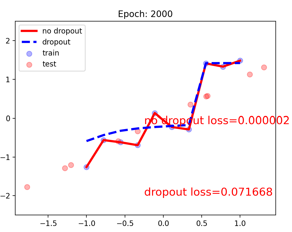
下面是对比使用dropout和不使用模型结果,与weight decay效果类似。
1 | import matplotlib.pyplot as plt |
这里的注意点:
- dropout加在激活函数层之后,下一层网络层之前;
- 最后一层输出之前要看情况增加dropout,对于简单的任务可以添加,复杂的任务可以不加;
- 务必使用
net.eval()和net.train()区分模型测试和训练。
Batch Normalization
批:一批数据,通常为mini-batch
标准化:0均值,1方差
优点:
- 可以用更大学习率,加速模型收敛;
- 可以不用精心设计权值初始化;
- 可以不用dropout或使用较小的dropout;
- 可以不用
L2或者使用较小的weight decay; - 可以不用
LRN(local response normalization)。
参考论文:《Batch Normalization Accelerating Deep Network Training by Reducing Internal Covariate Shift》
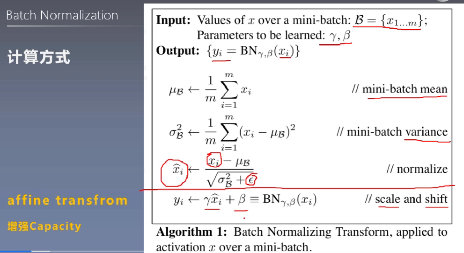
在Pytorch中Batch Normalization的实现方式
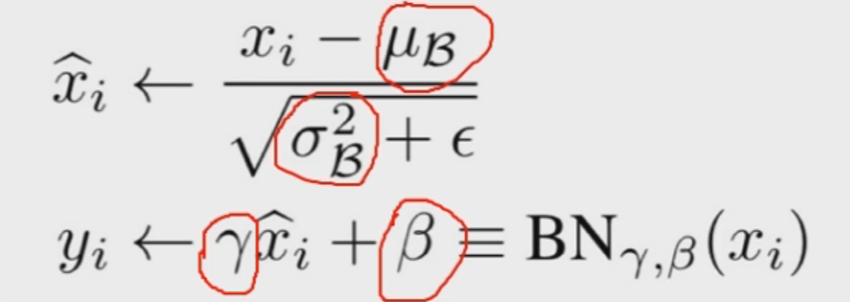
affine transform是指公式中增加了γ和β的计算方式
通过提出Batch Normalization的论文标题,我们可以知道其是为了解决ICS问题,我们在权值初始化部分就已经了解到:
下一层神经元的输出值方差与三个因素有关,(1)每一层神经元的数量;(2)输入值x的方差;(3)权重矩阵W的方差。
如果想要控制神经元的输出值方差为1,我们可以保证X的方差为1,若想要消掉n,那就是要W的方差为1/n。
而这里面通过增加Batch Normalization层,可以直接将每一层的输出进行归一化,从而无需精心设计权值初始化。但是其不仅解决了这一问题,还带来了其他优点。
下面我们通过代码来观察BN层的效果,还记得在权值初始化的部分,我们使用一个一百层的网络,并且加上激活函数,假设激活函数为Relu,如果我们不进行权值初始化,那么随着网络的加深,输出值会变成无穷小,如果我们对权值初始化的方法是将均值设置为0,方差设置为1,那么随着网络的加深,输出值会变成无穷大。解决这一问题是使用Kaiming初始化方法。那么如果我们直接使用BN层,结果会怎么样呢?
1 | import torch.nn as nn |
通过结果可以发现,无论是否对权值进行初始化,或者怎么样的初始化方法,只要使用了BN层,网络的输出方差就会处于一个非常稳定的值。
Pytorch中的_BatchNorm
nn.BatchNorm1dnn.BatchNorm2dnn.BatchNorm3d参数:
num_features:一个样本特征数量(最重要)eps:分母修正项- momentum:指数加权平均估计当前mean/var
- affine:是否需要affine transform
- track_running_stats:是训练状态,还是测试状态
主要属性:
- running_mean:均值
- running_var:方差
weight:affine transform中的gamma(γ)bias:affine transform中的beta(β)
这里的weight和bias是在训练中学习的,均值和方差在测试时,为当前的统计值,在训练时采用指数加权平均计算:
running_mean = (1-momentum) * pre_running_mean + momentum * mean_t
running_var = (1-momentum) * pre_running_var + momentum * var_t
pre_running_mean表示上一时刻的均值,mean_t表示当前时刻的均值。
1d、2d和3d的区别和使用
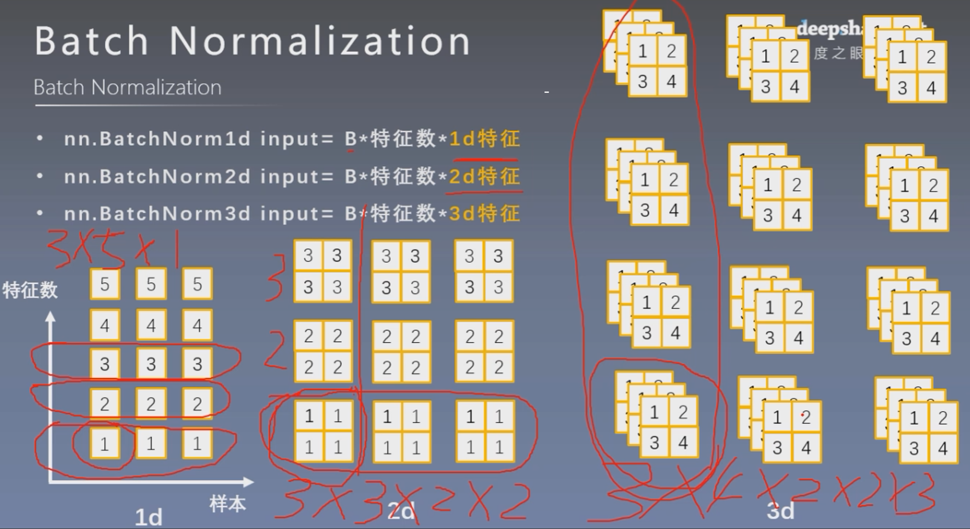
1 | # nn.BatchNorm1d |
这里计算均值和方差时,将同一批次样本的同一特征在一起计算,iteration=0时,每个样本的第一个特征值均为1,所以其均值为1,方差为0,而且因为是第一轮迭代,所以上一时刻的均值和方差默认值为0,1
所以iteration=0时,第一个特征的均值 =(1-momentum) * 0 + momentum* 1 = 0.3
iteration=0时,第一个特征的方差= (1-momentum) * 1 + momentum * 0 = 0.7
iteration=0时,三个样本第二个特征的均值为2,方差为0,所以
第二个特征的均值=(1-momentum) * 0 + momentum * 2 = 0.6
第二个特征的方差=(1-momentum) * 1 + momentum * 0 = 0.7
1 | # BatchNorm2d |
可以看到这里均值,方差,权重以及偏置的维度都是3,因为BN是将不同样本的同一特征一起算均值等,所以维度与特征数一致。
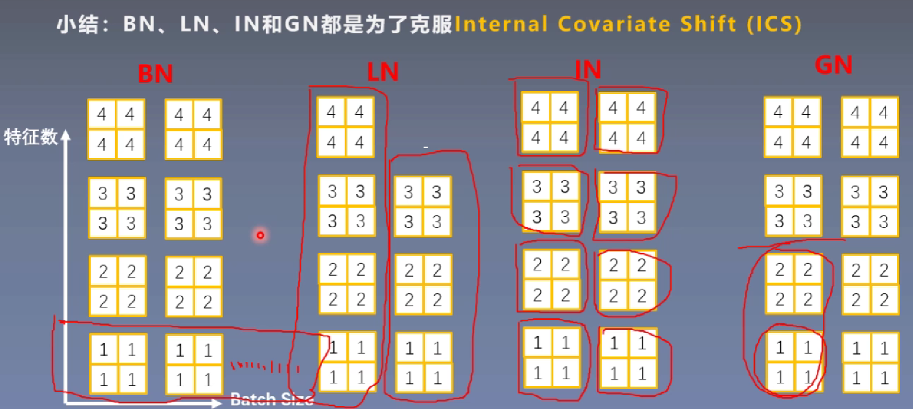
常见的Normalization in DL
Batch Normalization(BN)Layer Normalization(LN)Instance Normalization(IN)Group Normalization(GN)他们进行Normalization的方式均是如下方式
不同的点在于均值和方差的求取方式
Layer Normalization
起因:BN不适用于变长的网络,如RNN
思路:逐层计算均值和方差
注意事项:
- 不再有running_mean和running_var
- gamma和beta为逐元素的
nn.LayerNorm
主要参数:
normalized_shape:该层特征形状eps: 分母修正项elementwise_affine:是否需要affine transform
1 | # Layer Normalization |
这里weight和bias的size都是(3, 2, 2),因为每个样本都有3个特征且每个特征图为(2, 2),所以看出来LayerNorm更像是逐元素的计算均值和方差。(其实没咋搞懂每层的概念)
Instance Normalization
起因:BN在图像生成(Image Generation)中不适用
思路:逐Instance(channel)计算均值和方差
nn.InstanceNorm
主要参数:
num_features:一个样本特征数量(最重要)eps:分母修正项- momentum:指数加权平均估计当前mean/var
- affine:是否需要affine transform
- track_running_stats:是训练状态,还是测试状态
1 |
|
BatchNorm2d会将同一批次的同一特征,比如这里3个样本的第一个特征合并计算均值和方差,而Instance Normalization,会每个样本的每个特征图单独计算均值和方差。
Group Normalization
起因:小batch样本中,BN估计的值不准
思路:数据不够,通道来凑
注意事项:
- 不再有running_mean和running_var
- gamma和beta为逐通道(channel)的
应用场景:大模型(小batch size)任务
nn.GroupNorm
主要参数:
num_groups:分组数num_channels:通道数(特征数)eps:分母修正项affine:是否需要affine transform
1 | # group norm |